• #MakeoverMonday

    #MakeoverMonday Week 40 -US GDP by State

    It’s TC20 week! What an exciting time for the datafam. This is my first Tableau Conference since I’ve become more active in the community. I was supposed to go to TC Europe in London earlier this year but… the pandemic. So now TC20 is gonna have to be virtual again. But the cool thing about that is how many people from all over the world will be able to participate. I hope I’ll see you there!

    But let’s get to the topic this post is actually about: This week’s MakeoverMonday!
    Since it is TC20 week, there was also a special Live MakeoverMonday. I managed to join the Monday evening session on Youtube
    So what was different this week? Well, the idea is the same. But the topic was introduced on the livestream and we then had an hour to work with the dataset and submit our viz. After that, the MakeoverMonday team took some time to review some of the results on the livestream. So the big difference for me this week was timeboxing

    I usually don’t limit the time I work on my MakeoverMonday viz. And it often takes me quite a while. Typically it’s not because I lack the technical skills (though that happens too, of course). I typically have a hard time settling on an idea and tend to overthink things. But getting things done quickly is an important skill. So this was an interesting and exciting exercise for me!

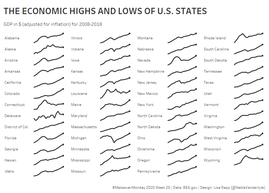
    So here’s what I ended up with after an hour:

    I’m actually quite surprised how much I like the result. It’s simple, you can easily compare different states and you can see some interesting patterns (check out Michigan’s 2008 dip, for example).

    How did I end up with that viz?
    I’ll let you in on a secret – it was a panicked last-ditch effort in the last 20 minutes or so. And isn’t that how it works quite often? How often do you start working with a dataset, build a viz, only to scratch it and try something else? I guess some people are well-organized, sketch out their vizzes in advance and actually stick to their plan. Well, I’m not one of those people. But in the end, you only see my finished viz and you don’t get to see all of my failed attempts. This week I’m going to change that and show you what happened before I settled on the final viz.

    A map showing the GDP of counties in the US.

    My first attempt was a simple map. I’ve never done a county-level map, so this seemed like a good dataset to try. However, the few very big values make the map pretty useless. And then you also have the usual problem of choropleth maps: Regions with small areas completely vanish. Do you see New York in that map? Me neither….

    My second attempt was a slope chart. I was hung up on that idea for quite some time. But as you can see it doesn’t work very well. There are way too many similar lines that overlap into a big mess and I don’t feel like you can gain any real insights from that chart.

  • #MakeoverMonday

    #MakeoverMonday Week 39 – Child Marriage

    THE PROCESS

    This week’s dataset consisted of only 4 fields: the country name, percentage of girls married by 15, percentage of girls married by 18 and percentage of boys married by 18. I decided to concentrate on the girls and not use the boys percentage. The next thing I noticed was that the girls married by 15 are a subset of the girls married by 18 and I wanted my viz to reflect that somehow. That’s how the idea of the squares within squares formed in my head.

    But how to get there?
    I knew I had to use polygons – something I’ve never really worked with before. Luckily, the Flerlage Twins are there to help you out with a handy blog post. Some data prep was needed (pivot the measure columns and quadruple the data to be able to draw the 4 corners of the square), do some calculations to get the positions of the corners – and voilà!

    Next, I had to get the country labels look nice. For that, I used another trick that was in Kevin’s blog post mentioned above: create the labels on a separate sheet and float them behind the polygon viz. I positioned the labels using transparent shapes – another trick I learned from the Flerlage’s blog. This has quickly become one of my favorite and most-used little tricks ever since I read the 14 use cases for transparent shapes blog post. 

    All that was left after that was implementing the sort functionality. I actually handled this in data prep by creating index fields based on the three sort options. Depending on the sorting parameter I would then use those indexes to calculate the X and Y position of each country in the small multiples grid. I then created the sort buttons and configured the parameter action.

    THE VERDICT

    All in all, I really liked how this turned out. It was really fun to try something new and explore polygons. I also rarely do small multiples, so that was a good opportunity for me to get more used to them. What’s also cool is that this was one of those cases where I had an idea in my head and I actually managed to recreate that exact idea – something that sadly doesn’t happen all the time. I do feel like this viz got more attention than I would usually get – so I guess other people out there liked it, too.

    However, let’s be very clear about something: This is not necessarily what I would call a best practice approach. Is it compelling to look at? I would say so. But is it the best way to communicate the data? Maybe not. Because check out the example on the right: If the white square is 100% – how much do you think the grey square represents? The correct answer is 76%! The first time I saw this I thought my calculations must be wrong. But I double-checked. They’re not. It’s just that we are super bad at estimating and comparing areas!